Best Deep Learning Tools to Buy in April 2026

Teaching for Deeper Learning: Tools to Engage Students in Meaning Making


Dive Into Deep Learning: Tools for Engagement


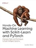
Hands-On Machine Learning with Scikit-Learn and PyTorch: Concepts, Tools, and Techniques to Build Intelligent Systems


Deep Learning for Biology: Harness AI to Solve Real-World Biology Problems


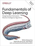
Fundamentals of Deep Learning: Designing Next-Generation Machine Intelligence Algorithms


Leveraging Deep Learning: Strategies and Tools for Assessment of Conceptual Understanding (Concepts in Action)


Backpropagation is an essential algorithm for training neural networks. It calculates the gradients of the loss function with respect to the model parameters, allowing us to update the parameters using an optimization algorithm like stochastic gradient descent (SGD). In PyTorch, backpropagation and parameter updates are seamlessly handled by the autograd package.
To perform backpropagation and update model parameters in PyTorch, follow these steps:
- Define the neural network model by creating a class that inherits from the nn.Module class. This class should have a forward method that defines how input tensors are transformed into output tensors. The parameters of the model should be defined as nn.Parameter objects.
- Initialize an instance of your model.
- Define a loss function that quantifies the difference between the predicted output and the expected output of your model. Common loss functions in PyTorch include nn.MSELoss (mean squared error) and nn.CrossEntropyLoss (cross-entropy loss).
- Create an optimizer object that will update the model parameters based on the computed gradients. PyTorch provides various optimizers, such as optim.SGD and optim.Adam. Initialize the optimizer with the model parameters and set the learning rate.
- For each training iteration: a. Clear the gradients of the model parameters using the zero_grad() method of the optimizer. b. Pass the input data through the model to obtain the predicted outputs. c. Calculate the loss by comparing the predicted outputs with the expected outputs. d. Call the backward() method on the loss tensor to compute the gradients of all model parameters. e. Update the model parameters by calling the step() method on the optimizer.
- Repeat the training iterations until convergence or a certain number of epochs.
By following these steps, PyTorch automatically performs backpropagation and updates the model parameters using the computed gradients. This process allows the model to gradually learn from the training data and improve its predictions.
What is a learning rate in neural networks?
The learning rate is a hyperparameter that determines the step size at which a neural network algorithm updates the weights and biases during the training process. It controls how fast or slow a neural network learns from the data.
A higher learning rate allows for larger updates in the weights and biases, which can lead to faster convergence but may also result in overshooting the optimal solution. On the other hand, a lower learning rate makes smaller updates, potentially improving the accuracy, but it can also make the training process slower.
Choosing an appropriate learning rate is crucial as it directly impacts the convergence and performance of the neural network. It often requires some experimentation and fine-tuning to find an optimal learning rate for a given task. Techniques like learning rate scheduling or adaptive learning rate methods can be used to improve the training process.
How to choose an appropriate activation function for a neural network?
Choosing an appropriate activation function for a neural network depends on several factors and considerations. Here are some guidelines to help you make that decision:
- Understand the problem: Gain a deep understanding of the problem you are trying to solve and the nature of your data. This will help you determine the characteristics that your activation function needs to possess.
- Non-linearity: Most neural networks require non-linear activation functions to introduce non-linearity into the model, allowing it to approximate complex functions. Linear activation functions will only produce linear outputs, limiting the network's capacity to learn complex patterns.
- Differentiability: To enable backpropagation, an activation function must be differentiable. This allows the gradients to be calculated, enabling efficient weight updates during training.
- Range of output: Consider the range of values that your activation function should produce. If your network requires outputs between 0 and 1 (e.g., for binary classification problems), sigmoid or softmax functions are suitable choices. If your problem involves regression tasks or unbounded outputs, functions like ReLU or identity functions can be used.
- Avoid vanishing or exploding gradients: Certain activation functions, such as sigmoid or hyperbolic tangent, are prone to vanishing or exploding gradients, especially in deep networks. This can result in slow convergence or even gradient explosion. Activation functions like ReLU or its variants (Leaky ReLU, Parametric ReLU) mitigate this issue to some extent.
- Specific requirements: Some tasks may have specific requirements that can be addressed by specific activation functions. For example, if the goal is to restrict a network's output to positive values, the Exponential Linear Unit (ELU) activation function could be chosen.
- Experimentation: Finally, it is always recommended to experiment with different activation functions and evaluate their impact on the network's performance using validation techniques. This helps determine which activation function best suits your specific task and dataset.
Remember, selecting an activation function is not a one-size-fits-all decision. It often requires some trial and error, along with an understanding of the problem and the behavior of different activation functions.
What are activation functions in neural networks?
Activation functions in neural networks determine the output of a neuron or a neural network model. They introduce non-linear behavior into the network, allowing it to learn complex patterns and better approximate complex functions. The activation function takes the weighted sum of inputs to a neuron and then decides whether the neuron should be activated or not based on a certain threshold. It is typically applied after the linear transformation of inputs by the weights and biases. Commonly used activation functions include sigmoid, tanh, ReLU, and softmax.
What is the role of activation regularization in neural networks?
Activation regularization is a regularization technique used in neural networks to prevent overfitting by regularizing the activations of the neurons.
In neural networks, activation refers to the output of each neuron in a layer. During training, each neuron learns to activate in response to specific inputs. However, in an overfit model, neurons may become too sensitive to specific inputs, leading to poor generalization on unseen data.
The role of activation regularization is to penalize or regularize the magnitudes of the neuron activations during training. It encourages the network to have smaller activation values, thus reducing the sensitivity of the neurons to specific inputs and promoting better generalization.
The activation regularization technique introduces an additional regularization term in the loss function, which measures the complexity or magnitude of the neuron activations. This regularization term is added to the overall loss during training, adjusting the learning process to encourage smaller activations.
By regularizing the activations, activation regularization helps prevent the network from overfitting the training data and improves its ability to generalize to unseen data. It provides a regularization mechanism specifically tailored to the behavior and sensitivity of individual neurons in the network.
What is gradient descent?
Gradient descent is an optimization algorithm used to minimize the cost function of a machine learning model. It is commonly used in training artificial neural networks.
In gradient descent, the algorithm iteratively adjusts the model's parameters in small steps in the direction of the steepest descent of the cost function. This is done by calculating the gradients (derivatives) of the cost function with respect to each parameter and updating the parameters in the opposite direction of the gradients.
The steps in gradient descent can be summarized as follows:
- Initialize the model's parameters with random values.
- Calculate the cost function, which quantifies the error between the predicted and actual values.
- Calculate the gradients of the cost function with respect to each parameter.
- Update the parameters by subtracting a small fraction (learning rate) of the gradients.
- Repeat steps 2-4 until the cost function converges or reaches a satisfactory level.
By continuously updating the parameters using the gradients, gradient descent can iteratively improve the model's performance and find the optimal values for the parameters that minimize the cost function.
How to install PyTorch on Windows?
To install PyTorch on Windows, follow these steps:
- Check if you have Python installed by opening a command prompt and running the command python --version. If Python is not installed, download and install it from the official Python website (https://www.python.org).
- Open a command prompt and install PyTorch using pip. Type the following command and press Enter: pip install torch torchvision torchaudio This command will install PyTorch along with the required dependencies.
- Once the installation is complete, test if PyTorch is installed correctly. Open a Python interpreter or a code editor and run the following code: import torch print(torch.__version__) If PyTorch is installed correctly, it will display the version number.
Congratulations! You have successfully installed PyTorch on Windows.
