Best Neural Network Toolkits to Buy in July 2026
Evolutionary Deep Learning: Genetic algorithms and neural networks


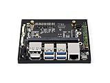
Waveshare NX Development Board Based On Jetson Xavier NX Alternative Solution for Jetson Xavier NX Developer Kit Carrier Board Only Can Directly Insert into Jetson Xavier NX Module
- SUPPORTS HIGH-RESOLUTION SENSORS FOR COMPLETE AI SYSTEMS.
- DIRECTLY COMPATIBLE WITH JETSON XAVIER NX MODULE.
- CLOUD-NATIVE SUPPORT FOR SEAMLESS AI DEPLOYMENT & UPDATES.

ChatGPT for Beginners: Prompt Engineering Made Easy

Beginner's Agentic AI Toolkit: LLM Agents, RAG Basics, and Simple Monetization Strategies – Entry-level

The All in One Agentic AI Bible: The Practical 7 Step Guide To Building Smarter AI Agents, Designing Goal-Oriented, LLM-Powered Systems That Think, Act, And Adapt In The Real World

Automated Machine Learning in Action

Applied AI and Blockchain for Sustainable Development (The Infinite Mind Toolkit Book 10)

Unlocking the Secrets of Prompt Engineering: Master the art of creative language generation to accelerate your journey from novice to pro
To implement a neural network in MATLAB, you can follow these steps:
- Define the architecture of the neural network: Determine the number of input and output nodes, as well as the number of hidden layers and nodes in each layer. This will depend on your specific problem.
- Create a neural network object: Use the feedforwardnet function to create a neural network object. Specify the architecture you defined in step 1 as input arguments.
- Prepare input-output data: Organize your input-output data into appropriate matrices or vectors. Each column of the input matrix represents one training example, and each column of the target matrix represents the desired output for that training example.
- Configure the neural network: You can set various parameters and properties of the neural network object using the configure function. This includes setting the transfer functions for each layer, defining training algorithms, etc.
- Train the neural network: Use the train function to train the neural network using your prepared input-output data. Choose an appropriate training algorithm (e.g., backpropagation).
- Test the neural network: Evaluate the performance of the trained network on a separate test dataset by passing the test inputs through the network and comparing the obtained outputs with the known targets.
- Use the trained network for predictions: Once your network is trained and tested, you can utilize it to make predictions on new, unseen data by simply passing the inputs through the network using the sim function.
- Fine-tuning and optimization: Depending on the performance of your network, you may need to fine-tune the architecture, training parameters, or data preprocessing techniques to achieve better results.
Remember, MATLAB offers various additional functions and capabilities for more advanced neural network tasks, such as regularization, hyperparameter tuning, and ensemble methods. Exploring the MATLAB documentation and examples will help you further enhance your neural network implementation.
What is the difference between gradient descent and stochastic gradient descent?
Gradient descent and stochastic gradient descent are both optimization algorithms used in machine learning to update the parameters of a model in order to minimize the error or loss function. The main difference between the two lies in the way they update the parameters during training.
Gradient Descent:
- In gradient descent, the parameters of the model are updated by computing the gradient (derivative) of the loss function with respect to each parameter.
- In each training iteration, the algorithm calculates the gradients for all training examples.
- The gradients are averaged across all examples, and the parameters are updated by taking a step in the opposite direction of the gradient, multiplied by a learning rate.
- This process is repeated until convergence or a specific number of iterations.
Stochastic Gradient Descent (SGD):
- In stochastic gradient descent, the parameters of the model are updated by computing the gradient (derivative) of the loss function for a single training example.
- In each training iteration, the algorithm randomly selects a single training example and calculates the gradient for that example only.
- The parameters are updated using the gradient computed for the single example, scaled by the learning rate.
- This process is repeated for each training example in a random order, and the algorithm typically goes through the entire dataset multiple times (known as an epoch).
- The randomness of example selection in each iteration makes the algorithm faster but noisier compared to batch gradient descent.
Overall, the main difference is that gradient descent calculates gradients for the entire dataset in each iteration, while stochastic gradient descent computes gradients for a single example or a small batch of examples at a time. Stochastic gradient descent is more computationally efficient but can be more prone to noise and slower convergence compared to gradient descent.
How to initialize the weights and biases in a neural network?
Initializing the weights and biases in a neural network is an important step that can affect the learning process and performance of the network. Here are some common methods for weight and bias initialization:
- Zero Initialization: Set all weights and biases to zero. Not recommended as it leads to symmetric neurons and all neurons in a given layer will learn the same features.
- Random Initialization: Initialize weights randomly from a Gaussian distribution with mean zero and a small variance. Initialize biases to zero or with a small constant. Commonly used for smaller networks.
- Xavier/Glorot Initialization: Initialize weights randomly from a Gaussian distribution with mean zero and a variance of (1 / (fan_in + fan_out)), where fan_in is the number of input neurons and fan_out is the number of output neurons of a given layer. Biases can be initialized to zero or with a small constant.
- He Initialization: Similar to Xavier initialization but with a variance of (2 / fan_in) instead of (1 / (fan_in + fan_out)). More suitable for networks using ReLU activation functions.
It's generally recommended to experiment with different weight initialization techniques to determine what works best for a specific neural network architecture and problem domain.
What is the role of activation functions in deep neural networks?
The role of activation functions in deep neural networks is to introduce non-linearity into the network and enable it to learn complex patterns and relationships in the data.
Activation functions are applied to the output of each neuron in a neural network. They take in the weighted sum of the inputs and apply a transformation to produce the output of the neuron. Without activation functions, the network would simply be a linear model that can only learn linear relationships.
Activation functions map the input values to a desired output range, typically between 0 and 1, or -1 and 1. Non-linear activation functions like sigmoid, tanh, or rectified linear units (ReLU) allow the network to model more complex relationships between inputs and outputs.
By introducing non-linearity, activation functions enable the network to learn and approximate arbitrary complex functions. This is important for tasks such as image recognition, natural language processing, and speech recognition, where the relationships between inputs and outputs are highly non-linear.
Choosing the right activation function is crucial as it can affect the network's performance, convergence speed, and overall accuracy. Different activation functions have different properties, and their choice depends on the specific problem and network architecture.
What is the purpose of the backpropagation algorithm?
The purpose of the backpropagation algorithm is to train artificial neural networks by updating the weights of the network's connections in order to minimize the error between the predicted output and the actual output. This algorithm calculates the gradient of the error function with respect to the weights in each layer, and then propagates this gradient information backwards through the network. This allows the algorithm to iteratively adjust the weights to improve the accuracy of the network's predictions. Ultimately, the backpropagation algorithm helps neural networks learn and adapt to make better predictions or decisions based on the provided data.